Catalan pseudo-primes

Posted by: Gary Ernest Davis on: May 16, 2011

In: Uncategorized
Comment!

0 Shares

Catalan pseudoprimes

As a special case of Fermat’s little theorem, if $p$ is an odd prime number then $2^p-2$ is divisible by $p$ , or, in the language of congruences, $2^p \equiv 2 (mod \phantom{.}p)$ .

The converse of this is not true: if $2^p \equiv 2 (mod \phantom{.}n)$ where $n$ is a positive integer, it does not follow that $n$ is prime. For example $n$ could be $561 = 3\times11\times 17$ . There are infinitely many such $n$ .

Composite integers that pass a test for prime numbers are commonly known as pseudoprimes. Of course whether a composite number is regarded as a pseuodprime depends on the particular prime number property we are using.

Another property of primes involves the Catalan numbers. These are the numbers $C_n$ defined by the recurrence relation $C_0=1$ and $C_{n+1}=C_0C_n+C_1C_{n-1}+\ldots+C_{n-1}C_1+C_nC_0 \textrm{ for } n \geq 0$ .

The Catalan numbers can also be defined recursively by $C_{n+1}=\frac{2(2n+1)}{n+2}C_n \textrm{ for } n\geq 0$ .

The Catalan numbers are the coefficients of $x$ in the series expansion of $\frac{1-\sqrt{1-4 x}}{2 x}=1 + x + 2x^2 + 5x^3 + 14x^4 + 42x^5 + 132x^6 + 429x^7 + 1430x^8 + 4862x^9 + 16796x^10+\ldots$

The Catalan numbers up to $C_{25}$ are

1, 1, 2, 5, 14, 42, 132, 429, 1430, 4862, 16796, 58786, 208012, 742900, 2674440, 9694845, 35357670, 129644790, 477638700, 1767263190, 6564120420, 24466267020, 91482563640, 343059613650, 1289904147324, 4861946401452.

Clearly $C_n$ grows rapidly with $n$ . In fact $C_n \sim \frac{4^n}{n^{3/2}\sqrt{\pi}}$ in the sense that the ratio of $C_n$ to $\frac{4^n}{n^{3/2}\sqrt{\pi}}$ approaches 1 as $n \to \infty$ :

Theorem 2 of Aebi & Cairns (see below) provides a property of prime numbers in terms of Catalan numbers:

If $p$ is an odd prime, then $(-1)^{\frac{p-1}{2}} .C_{\frac{p-1}{ 2} }\equiv 2 (mod \phantom{.}p)$

On the other hand, there are numbers other than primes that also have this property, for example $p=5907 = 3\times11\times179$ .

Aebi & Cairns call a composite number $n$ a Catalan pseudoprime if $(-1)^{\frac{n-1}{2}} .C_{\frac{n-1}{ 2} }\equiv 2 (mod \phantom{.}n)$ . Thus, 5907 is a Catalan pseudoprime.

Currently the only known Catalan pseudoprimes are:

$5907=3 \times 11\times179$
$1093^2 = 1093 \times 1093$
$3511^2 = 3511 \times 351$

The following two lines of MathematicaÂ® code:

n = 1;
While[Or[Mod[(-1)^((n – 1)/2)*CatalanNumber[(n – 1)/2], n] != 2, PrimeQ[n] == True], n = n + 2]

found 5907 in 1.86 seconds.

Beyond that things are much more difficult.

A related question

The Catalan numbers are related to the middle binomial coefficients $\left(\begin{array}{c c} n-1 \\ \ (n-1)/2 \end{array}\right)$ . When $n$ is odd, say $n =2k+1$ , we have $\left(\begin{array}{c c} n-1 \\ \ (n-1)/2 \end{array}\right) = \left(\begin{array}{c c} 2k \\ \ k \end{array}\right)$ . A theorem of ErdÃ¶s (see Finch, 2007, below) shows that almost always the middle binomial coefficient $\left(\begin{array}{c c} 2k \\ \ k \end{array}\right)$ is divisible by high powers of small primes. Let $g(k)$ denote the smallest odd prime dividing $\left(\begin{array}{c c} 2k \\ \ k \end{array}\right)$ . How does $g(k)$ vary with k? A plot of $g(k) \textrm{ versus } k \textrm{ for } 2\leq k\leq 10000$ is shown below.

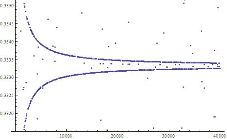
This plot indicates that although $g(k) =3$ commonly, there are values of k for which $g(k)$ becomes much larger. In light of the theorem of ErdÃ¶s cited above, a fundamental question is whether the numbers $g(k)$ stay bounded as k increases.

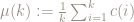
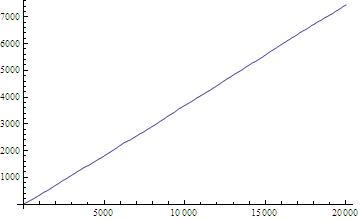
The plot below shows the running average of the values of $g(k)$ . It indicates that, possibly, $lim_{k\to\infty}\frac{1}{k}(g(2)+\ldots+g(k))=3$ .

Behavior of a number-theoretic function

The function $c(k) :=(-1)^k \left(\begin{array}{c c} 2k \\ \ k \end{array}\right)\phantom{.}(mod \phantom{.} 2k+1)$ takes the value 1 exactly when $2k+1$ is prime or a Catalan pseudoprime. How does $c(k)$ behave as a function of $k$ ?

A plot of $c(k) \textrm{ for } 1 \leq k \leq 5000$ , below, indicates that $c(k)$ is bounded above by a linear function of $k$ but has wide variation:

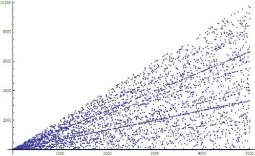
A plot for $1\leq k \leq 20000$ shows similar behavior, but appears more dense on the same scale:

This is more or less what we would expect if the values of $c(k)$ distributed themselves relatively uniformly across the remainders $mod \phantom{.} 2k+1$ . A plot of the running average $\mu(k):=\frac{1}{k}\sum_{i=1}^k c(i)$ , and of the running standard deviation $\sigma(k):=\sqrt{\frac{1}{k}\sum_{i=1}^k(c(i)-\mu(k))^2}$ , indicates a linear increase with $k$ :

Running average of c(k)

How does the function 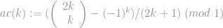$ac(k) :=(\left(\begin{array}{c c} 2k \\ \ k \end{array}\right) - (-1)^k )/(2k+1) \phantom{.}(mod \phantom{.} 1)$ behave as a function of $2k+1$ ? The plot below indicates that the values are not uniformly distributed:

A blow-up around the value $\frac{1}{3}$ shows the following behavior:

Similar behavior holds around the value $\frac{2}{3}$ .

Similar, but weaker, behavior occurs around the values $\frac{1}{5} \textrm{ and } \frac{1}{7}$ :

References & readings

Christian Aebi & Grant Cairns. Catalan numbers, primes and twin primes. (cairns_catalan)
Campbell, D. The Computation of Catalan Numbers. Math. Mag. 57, 195-208, 1984
Steven Finch (March 28, 2007)Central Binomial Coefficients (central_binomial_coefficients_finch)
Tom Davis (2006) Catalan Numbers (catalan_numbers1)
David Fowler, The Binomial Coefficient Function. The American Mathematical Monthly, Vol. 103, No. 1 (Jan., 1996), pp. 1-17.
W. Sander, A Story of Binomial Coefficients and Primes, The American Mathematical Monthly, Vol. 102, No. 9 (Nov., 1995), pp. 802-807
Keith Ball (2006). Strange Curves, Counting Rabbits, & Other Mathematical Explorations. Princeton University Press. ISBN-13: 978-0691127972

Tags: Catalan number, prime number, pseudo-prime

Republic of Mathematics blog

Catalan pseudo-primes