John Wilder Tukey introduced a five-number summary of a data set in 1969 his book Exploratory Data Analysis.

For a given data set, a five-number summary consists of:

• The median of the data
• The upper and lower quartiles of the data
• The minimum value of the data
• The maximum value of the data

The median of a numerical data set is a number m such that the number of data points less than m is the same as the number of data points greater than m.

For an odd number of data points, the median is chosen to be the middle data point, while for an even number of data points, the median is usually chosen to be the average of the two data points nearest the middle of the data.

The lower quartile splits the data below the median in the same way as the median splits the whole data set, and the upper quartile splits the data above the median in the same way.

A more formal definition of the median of a set of numerical data is that it is the number that minimizes

as a function of . In other words, for all we have:

 A five-number summary is a built-in function in R where it is called as summary(), although this R five-number summary is really a six-number summary since it includes the mean as well as the median of the data.

On that note, prior to Tukey, Arthur Lyon Bowley, in 1915, used a seven-number summary, consisting of the deciles in addition to the median, upper and lower quartiles, and the minimum and maximum.

A five-number summary of data is often presented in visual format as a box and whisker plot in which the bottom and top of the box are the first and third quartiles, and a line inside the box indicates the median. Whiskers extending from the top and bottom of the box are used to represent a variety of aspects of the data including the maximum and minimum values of the data, or one standard deviation above and below the mean. In the latter case, data not included in the whiskers is often indicated as an outlier by a dot.

In R, a boxplot for a data set can be produced using the boxplot() function. For example, with the data for birth weights (in ounces) of babies of a a sample of mothers who did not smoke during pregnancy (details posted here) , we get the following boxplot in R, using the code boxplot(nosmokedata,range=1.5)

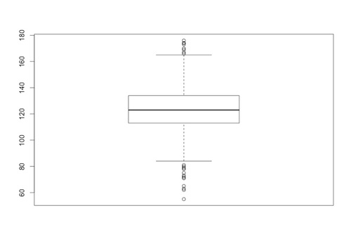
The specification range determines how far the whiskers extend from the box: a range of 1.5 means that the whiskers extend to the extreme data point that is no more than 1.5 times the interquartile range (the difference between the upper and lower quartiles) from the box.

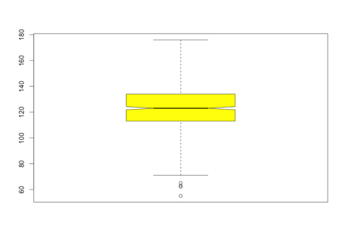
There are various options to the boxplot() function that allow us to jazz up the resulting image. For example, we can add color and a notch in the box to indicate the median more clearly. In the following we have done that and also increased the range to 2:

 The input to the boxplot() function in R is either a vector or a data frame. Using a data frame allows us to do a box and whisker plot, on the same output image, for more than one data set.

There is one proviso, however: the data sets have to be the same length to incorporate them into a data frame. What happens when we have related data sets that are of different lengths?

For example, the Stat Labs Data Page also has data on birth weights of babies of mothers who smoked during pregnancy, and that data is not the same size as the data on the babies of non-smoking mothers.

How do we combine these two different size data sets into a data frame?

Fortunately for us, this problem has arisen often enough that the prodigious Hadley Wickham has written a useful package called plry, that, among other things, will combine data sets of different lengths into a single data frame.

When you are using RStudio, for example, you can load the plyr package into R using the command install.packages(‘plyr’).

With the ply package installed, you call it using the library command library(plyr).

The plyr package is now ready to be used, and for our purposes we will utilize the r.bind.fill() function in the plyr package.

The function r.bind() can be used to join two data vectors of the same length into a data frame: it does not require the plyr package. The r.bind.fill() function in the plyr package creates two new data sets, each of total length equal to the sum of the lengths of the original data sets, and places NA values after the first data set, and before the second data set:

and

 and then uses r.bind() to combine these two modified data sets into a single data frame.

After importing the data on birth weights of babies of mothers who smoked during pregnancy –  smoke.data – we used r.bind.fill() to combine these two data sets into a data frame:

> combined<-rbind.fill(nosmokedata,smokedata)

and then used the boxplot() function with the data frame combined as input to plot both box plots together:

> boxplot(combined, ylab=”Birthweight(ounces)”, col=c(“royalblue2″,”red”))

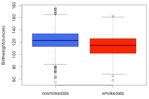
Here we have colored the boxes differently for visual distinction, and labelled the vertical axis.

This is a basic skill in descriptive and exploratory data analysis – something that should be carried out for all data sets you encounter.

As a wanna-be, or practicing, data analyst it’s a skill you need at your fingertips. It is basic and, like all basic skills, should be practiced regularly.

 Further Reading

x

Box-plot with R – Tutorial from R Bloggers,  by Fabio Veronesi