Data analysis: is it easier in Mathematica® ?
Posted by: Gary Ernest Davis on: June 12, 2015
I wrote a post yesterday on defining functions in R for beginners. By “beginners” I mean either people who are just learning R, or are just starting out in data analysis, or both.
Today I want to show how this might be easier  to do in Mathematica®.
First let’s define the function zsf[data,k] which calculates the proportion of data that lies within k standard deviations of the mean of the given data set:
zsf[data_, k_] := Length[Cases[data, x_ /; Abs[x – mean[data]] <= k*StandardDeviation[data]]]/Length[data]
The code “Cases[data, x_ /; Abs[x – mean[data]] <= k*StandardDeviation[data]]” keeps those instances, called x, of the data set that are within k standard deviations of the mean of the data.
As in R, we import the data as a text file from a URL:
nosmokedata = Import[“http://www.blog.republicofmath.com/wp-content/uploads/2015/\06/nosmoke.txt”, “List”]
The “List” option tells Mathematica® to import the data string as a formatted (ordered) list, which in R would be seen as a vector.
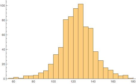
We plot a histogram of the data:
Histogram[nosmokedata]
We calculate the fraction of data that lies within 1 standard deviation of the mean and express that both as a fraction and a floating point number:
zsf[nosmokedata, 1]
N[%]
270/371
0.727763
Then we plot zsf[k] as a function of k over the range 0 through 4, subdivided into 20 equal intervals, as well as present the results in table form:
T = Table[{N[k], N[zsf[nosmokedata, k]]}, {k, 0, 4, 4/20}];
TableForm[T, TableHeadings -> {None, {“k”, “zsf[k]”}}]
ListPlot[T, Joined -> True, Mesh -> All]
![zsf[k] versus k](http://www.blog.republicofmath.com/wp-content/uploads/2015/06/zsfk-versus-k1.jpg)
![zsf[k] table](http://www.blog.republicofmath.com/wp-content/uploads/2015/06/zsfk-table.jpg)
Well, that’s it … the result could have been written very nicely in Mathematica® and saved as a PDF, or as a CDF and placed as an interactive document on the Web.
R has similar capabilities, so you pays your money and takes your choices.
I just feel data analysts should be aware there is a choice.
Now if Wolfram (Steve) could lower the price of Mathematica® to $50 …
Data analysis: R functions for beginners
Posted by: Gary Ernest Davis on: June 11, 2015
x
What is a function, anyway?
x
For programming purposes, one should think of a function as a type of object that takes certain types of INPUTS, and – once those inputs are given – produces a definite OUTPUT.
A simple example is the AVERAGE function, for which the input is a list of numbers

and the output is the average

We can think of the AVERAGE function schematically as follows:
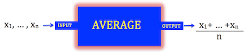
The “object” that acts as input to the function is a finite list of numeric data. The “object” that is output by the function is a single numeric value. The function itself is also an “object”.
Functions in R
x
You can define functions yourself in R using the function command. When you create a function it is an object, that can be used in R like any other object.
A function in R has 3 components:
- The function body. This is the entire code inside the function.
- The function arguments. These are the types of input needed for the function to work. They are specified in the body of the function.
- The function environment. This is a specification of the location of the inputs to the function.
The structure of a function will typically look like this:
functionname<-function(argument1, argument2, … ){computations using the arguments}
An example
In this example we use a function to compute the fraction of data points, from a given data set, that lie within 
We INPUTÂ a vector of numerical data 

Note that the input vector is a single object in R: it has numerical components, yet so far as R is concerned it is a column vector (= an ordered list).
We OUTPUT a single number:Â the fraction of data points, from
In specifying this function we will do something that is very common – we will make use of other, existing R functions, such as mean and standard deviation (among others).
Let’s see how this might work
Let’s name the function zsf (for “z-score function”).
So our definition will begin:
zsf<-function(argument1, argument2, … ){computations using the arguments}
and we have to fill in the arguments and the computations to get the output.
The function arguments will be a column vector and a numeric value. Let’s call the data vector argument data, and the numeric argument k:
zsf<-function(data, k){computations using the arguments}
To do the computation in the body of the function we have to compute the mean and standard deviation of the input data set:
mean(data), sd(data)
Note that the functions mean and sd are part of the R stats package, which loads automatically when you open R.
Now we have to carry out the remaining computations that will give us the output:
- First, we extract from the data those data points that are within k standard deviations of the mean m. We do this using the built-in subset and abs function:
subset(data, abs(data-mean(data))<=k*sd(data))
- Then we want the ratio of the size of this data subset to the full data set:
length(subset(data, abs(data-mean(data))<=k*sd(data)))/length(data)
Stringing this together, the final form for the function is:
zsf<-function(data, k){length(subset(data, abs(data-mean(data))<=k*sd(data)))/length(data)}
Realizing the function in R
To realize this function in R we first need to import a data set. Here is a data set consisting of birth weights, in ounces, of babies of mothers who did not smoke during pregnancy, taken from the Stat Labs Data Page, and formatted as a .txt file:Â nosmoke
By right-clicking on the “nosmoke” file link you can get the URL of this file, which is http://www.blog.republicofmath.com/wp-content/uploads/2015/06/nosmoke.txt
We import this data into R, name it “nosmoke” and define the z-score function as above, and use it to  compute what fraction of the data is within 1 standard deviation of the mean:
- First, the read.table command reads in the nosmoke data, which has no header row, and for which we have blank separators:
> nosmoke<-read.table(“http://www.blog.republicofmath.com/wp-content/uploads/2015/06/nosmoke.txt”, header=FALSE, sep=””)
- However, when R reads the data into memory in this format, it is a data frame and not a simple column vector. You can see this by entering:
> str(nosmoke)
to get the structure of the data frame “nosmoke”. You will see in the structure of the data frame a header for the birth weights. In our case the header, given by R, is ‘V1’:
‘data.frame’: 742 obs. of 1 variable:
$ V1: int 120 113 123 136 138 132 120 140 114 115 …
We can extract the column headed ‘V1’ as follows:
> nosmokedata=nosmoke[[‘V1’]]
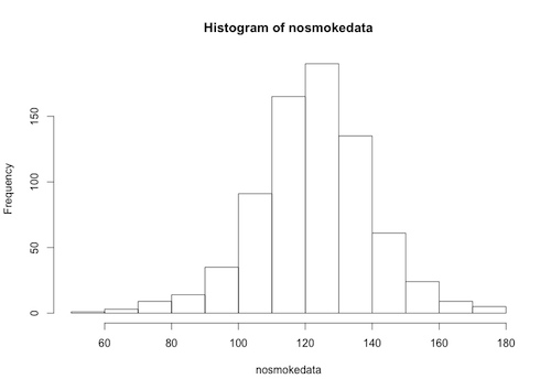
The “nosmokedata” is now a column vector, and we can, for example, plot a histogram of this data:
> hist(nosmokedata)
- Now we define the z-score function:
> zsf<-function(data,k){length(subset(data,abs(data-mean(data))<=k*sd(data)))/length(data)}
- And then we use the function to calculate what fraction of the data is within 1 standard deviation of the mean:
> zsf(nosmokedata,1)
[1] 0.7277628
So, approximately 72.8% of the data is within 1 standard deviation of the mean.
Plotting the function
Given a data set, such as the “nosmokedata” above, we can vary k and plot the fraction of data within k standard deviations of the mean, as simply a function of k (with the data as a given: in other words, with the data argument fixed).
- First we need to calculate a potential range of values for the variable k.
We calculate:
> (mean(nosmokedata)-min(nosmokedata))/sd(nosmokedata)
[1] 3.911052
and
> (max(nosmokedata)-mean(nosmokedata))/sd(nosmokedata)
[1] 3.043495
and so see that all the data lies within 4 standard deviations of the mean.
- We then create a vector of possible values for k using the seq function:
> values<-seq(0, 4, by=4/20)
Here we have chosen the range from 0 through 4, and divided that into 20 equally spaced intervals. A readout shows us the computed range of k values:
> values
[1] 0.0 0.2 0.4 0.6 0.8 1.0 1.2 1.4 1.6 1.8 2.0 2.2 2.4 2.6 2.8 3.0 3.2 3.4 3.6 3.8 4.0
We check that “values” is a vector:
> is.vector(values)
[1] TRUE
- Now we apply a function of 1 variable, k, to this vector of values.
First we define the function of the variable k:
> func<-function(k){zsf(nosmokedata,k)}
Then we use the function lapply to create a list as a result of applying this function of 1 variable to the vector “values”, and we unlist the result to get a data frame:
> y=unlist(lapply(values, func))
- We combine these two data frames with the cbind function, to get a data frame of k values paired with zsf(nosmokedata, k) values, and then plot that data frame:
> pairs<-cbind(values,z)
> plot(pairs,type=”b”,main=”zsf(k) as a function of k”, xlab=”k”, ylab=”zsf(k)”)
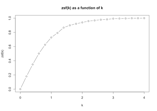
The plot allows us to see visually how the proportion of data within k standard deviations of the mean varies with k.
Note: the option type=“b” in the plot function draws both points and lines.
A skilled R programmer could have done this quicker and slicker: I hope I have laid out enough information so that you can see how functions are defined, can be applied to vectors, and plotted to give useful visual information.
Saving the function
Having defined a function such as the zsf function above, we would like to save it for future use.
Customizing R at Quick R byRob Kabacoff has a useful discussion on loading user-defined functions into R on startup.
Further reading
x
- User-written Functions from Quick R by Rob Kabacoff
- Functions from Advanced R by Hadley Wickham